Small values in wide integer columns: what ClickHouse, Snowflake, BigQuery, Redshift and Parquet actually store

A question came up while modeling a ClickHouse table. The column holds counts. Almost every value is under 256, a handful per million are in the billions, and nothing is negative. The tempting move is to be clever about it: declare Variant(Int8, Int64), cast small values into the small type at ingestion, and let the rare large ones take the wide path. The standard advice is the opposite: pick the smallest type that fits the whole column, which here means UInt64, and let a codec such as T64 do the saving.

The standard advice is right, but the reasons are more interesting than “codecs are good”, and they differ a lot between engines. Snowflake won’t let you choose a width at all. BigQuery charges you the full width no matter what. Redshift ships the “mostly small” idea as a built-in encoding. Parquet takes its own position, and DuckDB narrows your types behind your back.

This post goes through what each engine actually stores, where the width costs you, and when it is worth doing anything about it. The ClickHouse and DuckDB numbers come from experiments I ran on ClickHouse 24.12 and DuckDB 1.4 on an M1 Max. The rest come from each vendor’s documentation.

Three places where width costs

It helps to separate the logical width of a type (what the schema says, 8 bytes for Int64) from the physical width (how many bits a value actually occupies somewhere). A value pays in three places, and each engine lets a different set of them shrink:

1. At rest. Bytes on disk or object storage, after encoding and compression. This is where codecs work, and it is the layer almost every engine optimizes well.
2. In flight inside a query. Once a block is decompressed, it usually sits in memory at the logical width. Hash tables for GROUP BY and JOIN, sort buffers, the in-memory primary index and the number of values per SIMD register all follow the declared type.
3. At the boundaries. Network transfer between shards, spill to disk, temporary tables, and in BigQuery’s case the bill. Some of these are compressed and some are not.

A codec only fixes the first one. Most of the confusion about whether Int8 versus Int64 matters comes from looking at one layer and assuming it covers the other two.

ClickHouse: codecs at rest, full width in memory

The unit of compression is a block, not a column

ClickHouse writes each column of a part as a stream of compressed blocks. A block collects between min_compress_block_size (64 KiB) and max_compress_block_size (1 MiB) of uncompressed data, which for a UInt64 column is typically one granule of 8,192 rows. Each block carries a small header naming the codec, and the column’s codec chain runs block by block. A chain like CODEC(T64, ZSTD(1)) first applies the specialized transform, then hands its output to the general compressor.

That block boundary is what decides how outliers behave, so keep it in mind.

How T64 works

T64 is the integer-specific codec, and it’s short enough to describe completely.

For each block, T64 computes the min and max, then XORs them. The position of the highest set bit in min XOR max is the number of bits that ever change inside the block. Every bit above that is identical in every value, because it is identical in the two extremes. For signed types it handles the sign so that a range like [-128, 127] still comes out at 8 bits.

It then takes the values 64 at a time, treats them as a 64 by 64 bit matrix, and transposes it. Row i of the result holds bit i of all 64 values. It writes only the low rows that can vary and drops the rest. On read, it transposes back and fills the dropped high bits from the stored min.

 64 values of a UInt64 block        after transpose, one row per bit plane
 v0  = 0000…0000 1011 0010          plane 0  = bit 0 of v0..v63   ┐
 v1  = 0000…0000 0111 1100          plane 1  = bit 1 of v0..v63   │ written
 …                                  …                             │ (8 planes)
 v63 = 0000…0000 1110 0001          plane 7  = bit 7 of v0..v63   ┘
                                    plane 8…63 = identical in every value, dropped

The output is still regular, so a general compressor after it usually shrinks it further. That is why T64 is normally chained with LZ4 or ZSTD.

Two consequences follow from “XOR of min and max”, and both are easy to get wrong.

It is not a frame of reference. T64 does not subtract the min. It keeps the bits below the highest one where min and max disagree. A range that straddles a power of two costs far more than its size suggests:

Values in the block	Range	T64 bits per value
1024 or 1025	1	1.04
1023 or 1024	1	11.04
0 to 255	255	8.04
-128 to 127 (Int64)	255	8.04

1023 is 0b01111111111 and 1024 is 0b10000000000. They disagree on 11 bits, so every value in the block pays 11. Values that hover around a boundary like this, such as status codes near 1000 or IDs just past a million, are a case where ZSTD alone beats T64. On the 1023/1024 column, ZSTD(1) came out at 3.2 bits per value, against T64’s 11.

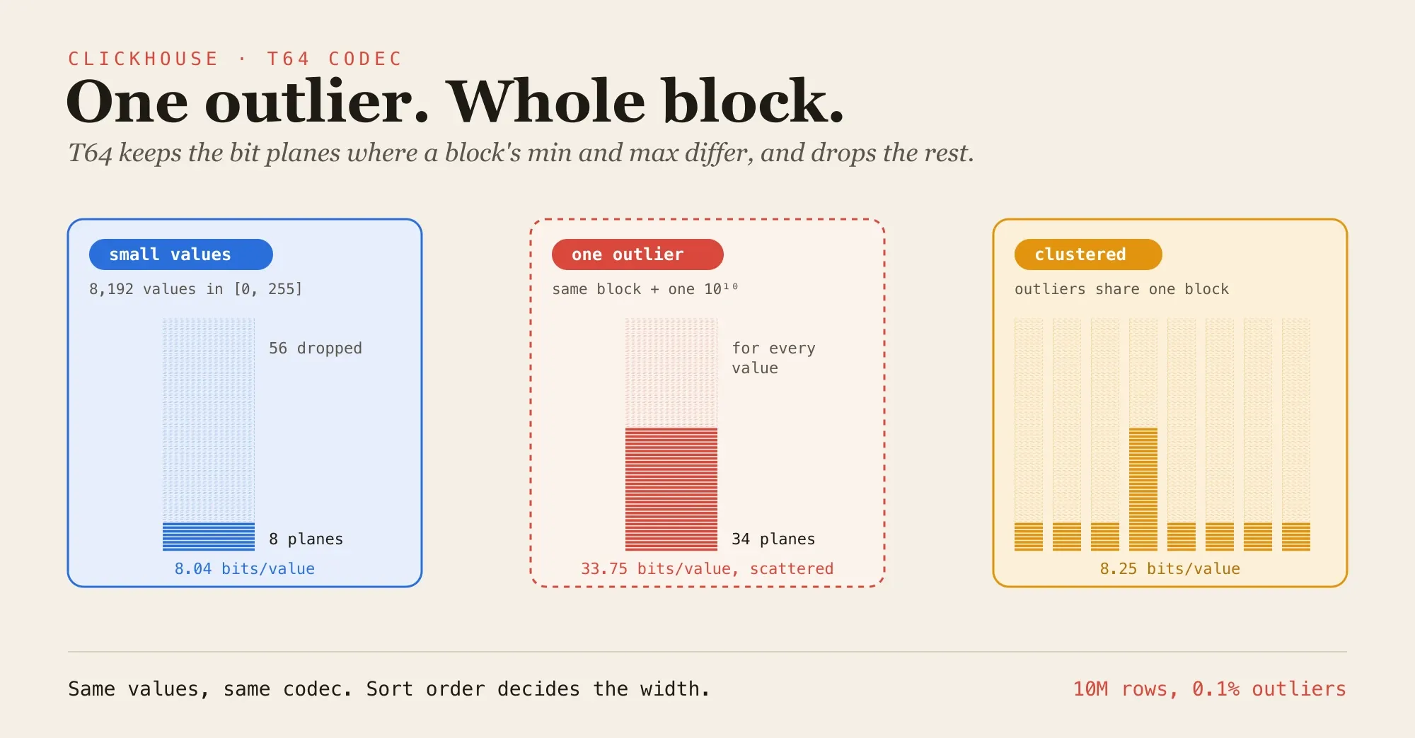
One outlier widens its whole block. This is the case the original question is about. A value of ten billion in a block of otherwise small numbers raises the width for all 8,192 values in that block, not just for itself. How much that costs depends entirely on where the outliers land:

10M UInt64 values	Raw T64, bits per value
Uniform in [0, 255]	8.04
Same, with 0.1% outliers up to 10¹⁰ at random positions	33.75
Same outliers, clustered in 1,000 row runs	8.25

With one outlier per thousand rows and about 8,000 rows per block, almost every block contains one, and the column behaves as if every value were 34 bits wide. Put the same outliers next to each other and only the few blocks that hold them pay. The sort order decides the compression ratio. If the large values correlate with something in your ORDER BY (a tenant, a device type, a date range), they cluster and T64 barely notices them.

What the general compressor recovers

The raw T64 numbers above are worst cases, because nobody runs T64 alone. Here is the full set for the same 10M rows, in bytes per value. Uniform values in [0, 255] have exactly 8 bits of entropy, so 1.0 is the floor:

Codec and type	Uniform [0, 255]	0.1% scattered outliers	Clustered outliers
UInt8, default LZ4	1.00	does not fit	does not fit
UInt64, default LZ4	3.04	3.05	not measured
UInt64 CODEC(ZSTD(1))	1.26	1.29	1.26
UInt64 CODEC(T64, LZ4)	1.01	1.15	1.02
UInt64 CODEC(T64, ZSTD(1))	1.01	1.06	1.01
Variant(UInt8, UInt64)	not measured	1.02	not measured

A few things stand out:

• UInt64 with T64 is within 1% of a native UInt8 when the values really are small. On disk, declaring the wide type costs essentially nothing.
• ZSTD behind T64 absorbs most of the outlier penalty. The extra bit planes in a widened block are almost all zeros, because only the outlier sets them, and ZSTD compresses long zero runs well. 34 raw bits per value become 8.5.
• The default LZ4 on an untouched UInt64 is the real waste. Three bytes per value for data with one byte of information. If you do nothing else, set a codec.

Other codecs in the same family attack different structure:

10M values	Codec	Bits per value
Multiples of 1,000 up to 255,000	T64, ZSTD(1)	16.3
	GCD, ZSTD(1)	10.1
Millisecond timestamps, 1s apart, with jitter	T64, ZSTD(1)	11.6
	Delta, ZSTD(1)	9.4
	DoubleDelta, ZSTD(1)	9.2

GCD divides every value in the block by their greatest common divisor, which removes zeros that T64 can’t see. Delta and DoubleDelta turn a steadily growing sequence into small differences. One thing I didn’t expect: on 24.12, CODEC(Delta, T64) and CODEC(GCD, T64) both fail at insert time with Cannot compress with T64 codec, data size … is not multiplier of 8. The first codec adds a header, which leaves T64 with input that isn’t a whole number of 8 byte values. Chain those with ZSTD or LZ4 instead.

Decompressed, everything is the logical width

This is the part the storage numbers hide. When a query reads a UInt64 column, the codec gives back 8 bytes per value, and every operator after that works on 8 bytes per value. I built a 100M row table with the same values stored twice, once in narrow types and once in UInt64, and ran each query five times, keeping the best:

Query over 100M rows	Narrow types	UInt64 everywhere	Cost of the wide type
sum(v)	0.029 s	0.058 s	2.0x time
GROUP BY k2, v, 256k groups	0.27 s, 187 MiB	0.45 s, 266 MiB	1.6x time, 1.4x memory
GROUP BY k1, k2, about 100M groups	2.47 s, 6.3 GiB	7.12 s, 8.7 GiB	2.9x time, 1.4x memory

Narrow types were UInt32 for k1 (up to 2M), UInt16 for k2 (up to 1,000) and UInt8 for v. The values were identical in both versions.

The sum difference is plain bandwidth: eight times the decompressed bytes and an eighth as many values per SIMD register. The GROUP BY difference is structural. ClickHouse picks a hash table layout from the key types. A single UInt8 or UInt16 key doesn’t get a hash table at all: it gets a flat array with 256 or 65,536 slots, indexed directly. Several fixed-width keys get packed into one integer of 32, 64, 128 or 256 bits and hashed as a single value. (UInt32, UInt16) is 6 bytes and packs into a 64-bit key. (UInt64, UInt64) needs 128 bits, which means bigger hash cells, more cache misses, and more memory for the same number of groups. The type you declare picks that code path, whatever the data looks like.

The same applies elsewhere:

• The primary index (primary.idx) keeps one entry per granule for every ORDER BY column, loaded in memory, at the logical width. On a table with billions of rows and a wide sort key, that is real RAM on every replica.
• Joins build their hash table at the key’s width, and a join between UInt32 and UInt64 keys pays a conversion first.
• Distributed queries send blocks between shards in ClickHouse’s Native format. That traffic is compressed with LZ4 by default, so it gets some of the at-rest benefit back, but the sender and receiver both hold full width blocks.

So the real advice is sharper than “the smallest type that fits”. It’s the smallest type that fits the whole column’s range, for the lifetime of the table. Storage barely cares. Query execution does.

Variant(Int8, Int64), examined properly

A Variant column in ClickHouse is stored as a discriminator stream (one UInt8 per row saying which type the row holds) plus one dense column per variant, containing only the rows of that type. In memory there’s also an offsets structure that maps each row to its position inside its variant’s column. On disk, a column that is 99.9% one type has a discriminator stream that compresses to almost nothing, and the small values sit in a genuinely 1-byte column.

That is why the unsigned form I measured, Variant(UInt8, UInt64), did well: 1.02 bytes per row against 1.06 for UInt64 with T64, ZSTD. It’s also where the good news ends.

ClickHouse refuses to create it. With the Variant type enabled, the table definition still fails:

Cannot create column with type 'Variant(Int64, Int8)' because variants 'Int64' and
'Int8' have similar types and working with values of these types may lead to
ambiguity. Consider using common single variant 'Int64' instead of these 2 variants
or set setting allow_suspicious_variant_types = 1 in order to allow it.

The engine is telling you what it thinks of the idea, and suggesting the alternative.

Arithmetic fails. SELECT x + 1 FROM v returns Illegal types Variant(Int64, Int8) and UInt8 of arguments of function plus. Every query has to either read the typed subcolumns (x.Int8, x.Int64, which are Nullable and NULL where the row holds the other type) or CAST(x AS Int64). Either way the value becomes an 8-byte integer before anything useful happens, so the in-memory cost is no better than a plain Int64 column, and you’ve added a discriminator read and a branch.

Ingestion has to choose for you. Parsing picks a variant per value, and the choice depends on the input format and settings. If one pipeline casts explicitly and another relies on inference, the same number can land in different variants in different parts. Queries that filter on one subcolumn then quietly miss the others.

It changes what the column means. Min/max skip indexes, partition keys, ORDER BY placement and comparisons all get harder to reason about on a Variant than on an integer.

Variant exists for columns that really do hold different kinds of values, such as a field that is sometimes a String and sometimes an Int64 in semi-structured data. As a storage trick for integer width it gains a few percent on disk, which T64 already delivers, and pays for it in every query.

If you really need the small path

When the outliers matter to storage and the queries mostly touch small values, there’s a more honest version of the same idea: two columns.

CREATE TABLE events
(
    ...
    count_small UInt8,                   -- the value when it fits, else 0
    count_large UInt64 CODEC(T64, ZSTD), -- the value when it doesn't, else 0
    count UInt64 ALIAS if(count_large = 0, count_small, count_large)
)

ClickHouse stores a column whose values are mostly defaults (by default, more than 93.75% zeros, controlled by ratio_of_defaults_for_sparse_serialization) in sparse serialization: only the non-default values and their positions. In a 1M row test with 0.1% outliers, count_large was stored Sparse at 0.05 bits per row, and queries that only need small values read a real UInt8. It’s more schema to maintain and every consumer has to use the alias, so reach for it only after measuring that the plain UInt64 is a problem.

Type semantics that bite when narrowing

Narrow types come with their own traps:

• Arithmetic widens, up to a point. toUInt8(200) + toUInt8(100) returns 300 as a UInt16, because ClickHouse promotes plus and multiply to the next width. sum() over a UInt8 returns UInt64. At the top of the range there’s nowhere left to go, and UInt64 arithmetic wraps without an error.
• CAST wraps silently. CAST(300 AS UInt8) is 44. Use accurateCast (throws) or accurateCastOrNull in ingestion paths that narrow.
• Narrowing later is a rewrite. ALTER TABLE … MODIFY COLUMN with a new type is a mutation that rewrites the column in every part. Changing only the codec is cheaper: new parts use it right away, and old parts pick it up as they are merged.
• LowCardinality over integers is blocked by default too (allow_suspicious_low_cardinality_types), because ClickHouse expects it to hurt performance. A plain integer with a codec is almost always smaller and faster.

Snowflake: no width to choose

Snowflake treats INT, INTEGER, BIGINT, SMALLINT, TINYINT and BYTEINT as synonyms for NUMBER(38, 0). Its documentation says plainly that precision doesn’t affect storage: NUMBER(2, 0) and NUMBER(38, 0) holding the same value take the same space. Instead, for each micro-partition (50 to 500 MB of uncompressed data), Snowflake looks at the column’s min and max and sizes every value in that partition from them.

That is the T64 idea applied automatically, at a much coarser grain. Outliers behave the same way: one huge value widens its micro-partition, and clustering decides how many partitions contain one. Since a micro-partition is far larger than a ClickHouse block, scattered outliers are harder to escape, and clustering keys are the tool to keep them together.

What Snowflake does with widths during execution isn’t documented in detail, so I won’t guess at it. The practical points:

• Don’t spend time on SMALLINT versus BIGINT. They are the same type.
• Scale does matter. Snowflake’s docs note that the number of digits after the decimal point affects storage. A NUMBER(38, 10) holding whole numbers is paying for precision it doesn’t use.
• Clustering is your outlier control. If large values correlate with a key you already cluster on, they cost you in few partitions. If they’re scattered, they cost you everywhere.

BigQuery: width is a billing unit

BigQuery has exactly one integer type, INT64, with INT, BIGINT, SMALLINT and the rest as aliases. There’s nothing to narrow.

The interesting part is billing. BigQuery charges queries by logical bytes scanned, and an INT64 value is 8 logical bytes whether it holds 0 or 9e18. Under on-demand pricing, a scan of a billion-row integer column is billed as 8 GB, however well the underlying Capacitor format compressed it. Storage is different: a dataset can switch to storage_billing_model = 'PHYSICAL' and pay for compressed bytes, which is where a mostly small column finally gets credit for being small.

So in BigQuery the width question turns into three others:

• Which columns does the query touch? With 8 bytes per value fixed, projection and partition or cluster pruning are the only levers on scan cost.
• Is physical storage billing cheaper for this dataset? For wide integer columns full of small values, it usually is, because compression ratios on that data are high. It doesn’t change query cost.
• Would a capacity reservation make scan volume irrelevant? Under slot-based pricing you pay for compute, not bytes, and the logical width stops mattering to the bill.

Redshift: the Variant idea as an encoding

Redshift offers SMALLINT, INTEGER and BIGINT at 2, 4 and 8 bytes, and a per-column compression encoding chosen at table creation or automatically with ENCODE AUTO.

Among those encodings are MOSTLY8, MOSTLY16 and MOSTLY32, which are exactly the idea from the start of this post, built in. On a BIGINT column with MOSTLY8, every value that fits in a signed byte is stored in one byte, and values that don’t are stored raw at full width. It’s a physical choice, invisible to queries: the column is still BIGINT everywhere in SQL, with no casts and no ambiguity. That’s the version of Variant(Int8, Int64) that makes sense, because the engine owns the mapping.

In practice you rarely need it. The default for integer types is AZ64, Amazon’s own SIMD-friendly encoding, which adapts to small values on its own and which AWS recommends ahead of the older encodings. Under automatic encoding, sort key columns are left RAW, because heavily compressed sort keys can make range-restricted scans perform poorly.

The width still matters in the other two layers. Redshift’s own guidance is to use the smallest column size that fits, because intermediate results of complex queries can land in temporary tables, which are not compressed. A column declared too wide costs memory and spill space during execution, however well it compresses at rest.

Parquet and the lakehouse: two physical widths and cheap widening

Parquet has only two physical integer types, INT32 and INT64. INT(8) and INT(16) are logical annotations on an INT32, so at the file format level there’s no 1 byte integer to choose. The encodings do the narrowing:

• Dictionary encoding (the default for most writers) stores the distinct values once and writes indexes with the RLE/bit-packing hybrid at ceil(log2(dictionary size)) bits each. A mostly small column with a few thousand distinct values encodes to a handful of bits per row, and outliers are just more dictionary entries. If the dictionary gets too big, writers fall back to plain encoding for the rest of the column chunk.
• DELTA_BINARY_PACKED splits values into blocks, 128 values in 4 miniblocks of 32 in the common writer configuration. It stores differences, subtracts the block’s minimum difference (a real frame of reference, unlike T64) and bit-packs each miniblock at its own width. An outlier inflates only its 32 value miniblock, a much smaller blast radius than a ClickHouse block or a Snowflake micro-partition.

Then comes whatever general compressor the writer chose (Snappy, ZSTD, LZ4) on top.

The lakehouse table formats add something the warehouses don’t: type widening as a metadata change. Iceberg allows promoting int to long without rewriting data files. Old files keep their INT32 columns and readers widen them on read. Recent Delta Lake releases support the same through the type widening feature, from byte up through long. That changes the risk calculation. On Iceberg you can start narrow and widen later for free, while on ClickHouse, widening is a mutation over every part.

Engines reading Parquet (Spark, Trino, DuckDB, ClickHouse itself) decode into their own in-memory formats at the declared width, so the execution-time costs from the ClickHouse section apply again once the data is loaded.

DuckDB: it narrows for you, twice

DuckDB is worth a look because it deals with both layers automatically.

At rest, DuckDB compresses each column segment within a row group of 122,880 rows. During checkpoint, it analyzes each segment and picks the best of several lightweight methods: constant, RLE, dictionary, bit-packing (with frame-of-reference and delta modes), FSST for strings, and ALP for floats. On the same 10M row data as above, a BIGINT column of values in [0, 255] was stored with BitPacking in 82 segments. The same column with 0.1% scattered outliers needed 163 segments for the same row count, also bit-packed: roughly double the storage, the same outlier widening effect at DuckDB’s own grain.

During execution, DuckDB applies an optimization called compressed materialization. Before operators that build large intermediate state, like hash aggregates and sorts, it uses column statistics to shift and cast integers into the narrowest type that holds their range, then undoes it on the way out. The plan for SELECT small, count(*) FROM t GROUP BY small over a BIGINT column shows it directly:

__internal_compress_integral_utinyint(#0, 0)     -- before the aggregate
__internal_decompress_integral_bigint(#0, 0)     -- after it

The hash table is built over 1 byte keys even though the column is BIGINT. That is exactly the gap the ClickHouse benchmark above measured, closed by the optimizer using min/max statistics. It’s only as good as the statistics. A single outlier widens the column’s range, and the narrowed type widens with it.

Druid and Pinot: dictionaries first

Real-time OLAP stores lean on dictionary encoding for dimensions. Pinot’s default forward index for dictionary-encoded columns is fixed-bit: each row stores a dictionary id at exactly as many bits as the column’s cardinality needs, so a long column with 200 distinct values costs 8 bits per row wherever the values fall. Druid dictionary-encodes string dimensions, and for numeric columns offers a longEncoding of auto, which picks a lookup table or offset encoding with variable bit width based on the data, or longs, which stores values as-is before compression. In both systems the logical type is still the wide one once the value leaves the index.

Side by side

Engine	Integer widths you declare	Who narrows at rest	Granularity of the width decision	Width during execution
ClickHouse	8 to 256 bits, signed and unsigned	You, via codecs (T64, Delta, GCD, ZSTD)	Compressed block, about 8K rows	Declared type
Snowflake	None, all NUMBER(38,0)	Engine, automatically	Micro-partition	Not documented
BigQuery	None, all INT64	Engine, invisibly	Capacitor internals	Billed at 8 bytes
Redshift	16, 32, 64 bits	Encoding (AZ64, MOSTLY*, DELTA)	1 MB block	Declared type, temp tables uncompressed
Parquet	32 or 64 physical bits	Encoding (dictionary, DELTA_BINARY_PACKED)	Miniblock of 32 values, or dictionary	Reader’s choice
DuckDB	8 to 128 bits	Engine, per segment	Column segment	Narrowed by statistics before aggregates and sorts

What I’d actually do

For the column in the original question, mostly under 256, occasionally in the billions, never negative, on ClickHouse:

value UInt64 CODEC(T64, ZSTD(1))

Then I’d check where the outliers land relative to the sort key, because that decides whether T64 works as intended.

More generally:

1. Declare the type from the range the column can ever hold, not the typical value. On disk the wide type is nearly free with a codec. Guessing too narrow and wrapping silently is far worse than paying a few percent.
2. Always set a codec on wide integer columns in ClickHouse. Default LZ4 on a UInt64 of small values was 3 bytes per value against 1 with T64. That’s the cheapest win in this post.
3. Narrow the types you group, join and sort by. That’s where logical width shows up as time and memory: 2.9x on a high cardinality GROUP BY. A dimension id that fits in UInt32 should be UInt32 if it’s in the ORDER BY or in every GROUP BY.
4. Let the sort order work for you. If outliers correlate with a sort key column, T64, Snowflake micro-partitions and DuckDB segments all pay only where the outliers are.
5. Pick the codec for the structure of the data. T64 for small ranges, GCD for common factors, Delta or DoubleDelta for sequences, plain ZSTD for a few repeated values or ranges that straddle a power of two. Try them against real data, not intuition.
6. Don’t use Variant for width. Use it when the values are genuinely different types. If storage for rare outliers is a proven problem, split into a small column and a sparse large column behind an alias.
7. On Snowflake and BigQuery, stop thinking about integer widths. Think about clustering, scale, projection and the billing model.

To check what a codec change actually did in ClickHouse, compare compressed and uncompressed bytes per column on the parts that hold data:

SELECT
    column,
    type,
    formatReadableSize(sum(column_data_compressed_bytes))   AS compressed,
    formatReadableSize(sum(column_data_uncompressed_bytes)) AS uncompressed,
    round(sum(column_data_compressed_bytes) * 8 / sum(rows), 2) AS bits_per_row
FROM system.parts_columns
WHERE database = 'default' AND table = 'events' AND active
GROUP BY column, type
ORDER BY sum(column_data_compressed_bytes) DESC;

Remember that old parts keep their old codec until they’re merged, so a fresh comparison needs either new data or an OPTIMIZE … FINAL on a copy.

The general lesson

“Use the smallest type” and “let compression handle it” sound like opposing advice, and they aren’t. They’re about different layers. Compression owns the bytes at rest, and in every engine here it is good enough that the declared width barely matters on disk. The declared width owns everything that happens after decompression: hash table layouts, index memory, SIMD throughput, spill, and, in BigQuery’s case, the invoice. The useful question for any column isn’t “how small can I make it”, it’s “which of the three layers is this column going to be expensive in”, and the answer is usually visible in the queries that touch it, not in the table definition.